The Nonequivalent Group Design
In this exercise you are going to create a nonequivalent group or an untreated control group design of the form
where each O indicates an observation or measure on a group of people, the X indicates the implementation of some treatment or program, separate lines are used to depict the two groups in the study, the N indicates that assignment to either the treatment or control group is not controlled by the researcher (the groups may be naturally formed or persons may self-select the group they are in), and the passage of time is indicated by moving from left to right. We will assume that we are comparing a program and comparison group (instead of two programs or different levels of the same program).
This design has several important characteristics. First, the design has pretest and posttest measures for all participants. Second, the design calls for two groups, one which gets some program or treatment and one which does not (termed the "program" and "comparison" groups respectively). Third, the two groups are nonequivalent, that is, we expect that they may differ prior to the study. Often, nonequivalent groups are simply two intact groups which are convenient to the researcher (e.g., two classrooms, two states, two cities, two mental health centers, etc.).
You will use the pretest and posttest scores from the first exercise as the basis for this exercise. The first thing you need to do is to copy the pretest scores from column 5 of Table 1-1 into column 2 of Table 3-1. Now, you have to divide the 50 participants into two nonequivalent groups. We can do this in several ways, but the simplest would be to consider the first 25 persons as being in the program group and the second 25 as being in the comparison group. The pretest and posttest scores of these 50 participants were formed from random rolls of pairs of dice. Be assured, that on average these two subgroups should have very similar pretest and posttest means. But in this exercise we want to assume that the two groups are nonequivalent and so we will have to make them nonequivalent. The easiest way to make the groups nonequivalent on the pretest is to add some constant value to all the pretest scores for persons in one of the groups. To see how you will do this, look at Table 3-1. You should have already copied the pretest scores (X) for each participant into column 2. Notice that column 3 of Table 3-1 has a number "5" in it for the first 25 participants and a "0" for the second set of 25 persons. These numbers describe the initial pretest differences between these groups (i.e., the groups are nonequivalent on the pretest). To create the pretest scores for this exercise add the pretest scores from column 2 to the constant values in column 3 and place the results in column 4 of Table 3-1 under the heading "Pretest (X) for Nonequivalent Groups". Note that the choice of a difference of 5 points between the groups was arbitrary. Also note that in this simulation we have let the program group have the pretest advantage of 5 points.
Now you need to create posttest scores. You should copy the posttest scores from column 6 of Table 1-1 directly into column 5 of Table 3-1. In this simulation, we will assume that the program has an effect and you will add 7 points to the posttest score of each person in the program group. In Table 3-1, the initial group difference (i.e., 5 points difference) is listed again in column 6 and the program effect or gain (i.e., 7 points) in column 7. Therefore, you get the final posttest score by adding the posttest score from the first exercise (column 5), the group differences (column 6) and the program effect or gain (column 7). The sum of these three components should be placed in column 8 of Table 3-1 labeled "Posttest Y for Nonequivalent Groups".
It is useful at this point to stop and consider what you have done. When you combine the measurement model from the first exercise with what you have done here, we can represent each person's pretest score with the formula
X = T + D + eX
where:
X = the pretest score for a person
T = the true ability or true score (based on the roll of a pair of dice)
D = initial group difference (D = 5 if the person is in the program group; D = 0 if in comparison group)
eX = pretest measurement error (based on the roll of a pair of dice)
Similarly, we can now represent the posttest for each person as
Y = T + D + G + eY
Y = the posttest score for a person
T = the same true ability as for the pretest
D = the same initial group difference as on the pretest
G = the effect of the program or the Gain (G = 7 for persons in the program; G = 0 for comparison persons)
eY = posttest measurement error (based on a different roll of the dice than pretest error)
It is important to get a visual impression of the data and so, as in the first two exercises, you should graph the univariate and bivariate distributions. Remember that as in the randomized experimental simulation you need to distinguish the program group scores from the comparison group scores on all graphs. Graph the pretest distribution in Figure 3-1, the posttest in Figure 3-2, and the bivariate distribution in Figure 3-3. As before, you should also estimate the central tendency in the univariate distributions, taking care to do this separately for each group. And, you should visually fit a line through the bivariate data, fitting separate lines for the program and comparison groups.
When all of this is completed you should be convinced of the following:
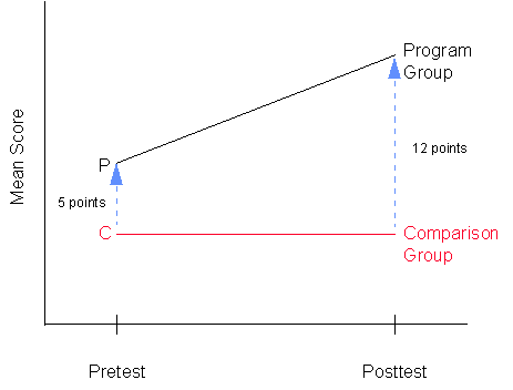
- There are differences between the program and comparison groups on the pretest. If you examine the pretest distributions in Figure 3-1, you should see that the central score for the program group is about 5 points higher than the central score of the comparison group (this is no surprise because you added in the 5 points). This difference is typical of what we expect when we use nonequivalent groups in research and simply tells us that prior to the study one group is higher than the other on the pretest characteristic.
- There are even larger differences between the groups on the posttest. In fact, the posttest difference between groups should be about 12 points (again, this is no surprise because you added in 5 + 7 points). If this were real data and you were going to analyze it, you would probably begin to suspect that your program may have had an effect because the posttest difference exceeds the pretest difference.
-
If you were to graph the central values for the pretest and posttest for the two groups, you would probably get a picture that looks something like this:

One alternative explanation (for a program effect) that you would have to consider is the possibility of a selection-maturation threat, that is, that your two groups are maturing at different rates. However, you know this is not the case because you specifically put in the same size group difference of 5 points on both the pretest and posttest (i.e., in the absence of the program, the groups did not mature at different rates). Nevertheless, if you were analyzing data like this in real life, you would have to assume that in the absence of the program the differences between the groups were the same on the pretest and posttest and that any additional difference (in this case 7 points) must be due to the program. You might know from previous research that a maturational pattern like the one in the above figure would be unlikely and rule out the threat as being improbable on that basis. Nevertheless, it should be apparent that you would be much better off, if you had a better idea of how the two groups would have changed from pre to post in the absence of the program. If you had taken an additional pretest observation (i.e. double pretest or the "dry run" experiment), you would have a much better idea of whether selection-maturation is a legitimate threat. In any event, you should be more firmly convinced of the importance of selection bias threats in nonequivalent group designs of this type.
- You should also note what would happen if you analyzed the data in other ways. Obviously a simple t-test of differences on the posttest would give an inappropriately large estimate of program effect — in this example, it would tell you that the groups differ by about 12 points, but you know that a good deal of that is due to initial differences. On the other hand, an analysis of variance (or t-test) on gain scores would work here but only because you know that without the program (i.e., if you had not added the 7 point program effect) the two groups would have gained, on the average, exactly the same amount (in this simulation, they would have gained nothing!). You should be convinced then that the analysis of variance on gain scores relies on the assumption of equal gain in both groups in the absence of the program.
- You have only simulated one possible outcome of many. You could, for example, simulate a null case (i.e., no effect of the program) simply by omitting the 7 points added to the program group persons. You could have a constant maturation rate by adding a constant value to all posttest scores. Or, you could simulate a selection-maturation problem by adding different constants to the posttest scores (or true scores) of the two groups. Or you could start out with an inferior program group by adding the group difference to the comparison group instead.
- Finally, you should also recognize an important fact about selection bias which is not illustrated in this exercise. When we select nonequivalent groups we expect that they may differ on one or more characteristics prior to the study. If we find that the pretest scores of our two groups are equal, we cannot assume that there is no selection bias or difference between the groups. The pretest averages could be equal by chance or the groups could differ on any number of other characteristics that are not measured by the pretest but nevertheless affect the posttest scores. We cannot conduct a t-test on pretest differences, find that there is no significant difference and conclude that selection bias is not a problem. Selection bias occurs whenever our groups differ on some pre-study characteristic that affects the posttest and when this pre-study difference is not perfectly described or "accounted for" by the difference on the pretest.
Nonequivalent Group Design — Table 3-1
| Person | Pretest X from Table 1-1 |
Pretest Group Difference |
Pretest (X) for Nonequivalent Groups |
Posttest Y from Table 1-1 |
Posttest Group Difference |
Effect of Program (G) |
Posttest (Y) for Nonequivalent Groups |
|---|---|---|---|---|---|---|---|
| 1 | 5 | 5 | 7 | ||||
| 2 | 5 | 5 | 7 | ||||
| 3 | 5 | 5 | 7 | ||||
| 4 | 5 | 5 | 7 | ||||
| 5 | 5 | 5 | 7 | ||||
| 6 | 5 | 5 | 7 | ||||
| 7 | 5 | 5 | 7 | ||||
| 8 | 5 | 5 | 7 | ||||
| 9 | 5 | 5 | 7 | ||||
| 10 | 5 | 5 | 7 | ||||
| 11 | 5 | 5 | 7 | ||||
| 12 | 5 | 5 | 7 | ||||
| 13 | 5 | 5 | 7 | ||||
| 14 | 5 | 5 | 7 | ||||
| 15 | 5 | 5 | 7 | ||||
| 16 | 5 | 5 | 7 | ||||
| 17 | 5 | 5 | 7 | ||||
| 18 | 5 | 5 | 7 | ||||
| 19 | 5 | 5 | 7 | ||||
| 20 | 5 | 5 | 7 | ||||
| 21 | 5 | 5 | 7 | ||||
| 22 | 5 | 5 | 7 | ||||
| 23 | 5 | 5 | 7 | ||||
| 24 | 5 | 5 | 7 | ||||
| 25 | 5 | 5 | 7 | ||||
| 26 | 0 | 0 | 0 | ||||
| 27 | 0 | 0 | 0 | ||||
| 28 | 0 | 0 | 0 | ||||
| 29 | 0 | 0 | 0 | ||||
| 30 | 0 | 0 | 0 | ||||
| 31 | 0 | 0 | 0 | ||||
| 32 | 0 | 0 | 0 | ||||
| 33 | 0 | 0 | 0 | ||||
| 34 | 0 | 0 | 0 | ||||
| 35 | 0 | 0 | 0 | ||||
| 36 | 0 | 0 | 0 | ||||
| 37 | 0 | 0 | 0 | ||||
| 38 | 0 | 0 | 0 | ||||
| 39 | 0 | 0 | 0 | ||||
| 40 | 0 | 0 | 0 | ||||
| 41 | 0 | 0 | 0 | ||||
| 42 | 0 | 0 | 0 | ||||
| 43 | 0 | 0 | 0 | ||||
| 44 | 0 | 0 | 0 | ||||
| 45 | 0 | 0 | 0 | ||||
| 46 | 0 | 0 | 0 | ||||
| 47 | 0 | 0 | 0 | ||||
| 48 | 0 | 0 | 0 | ||||
| 49 | 0 | 0 | 0 | ||||
| 50 | 0 | 0 | 0 |
Nonequivalent Group Design — Figure 3-1

Nonequivalent Group Design — Figure 3-2

Nonequivalent Group Design — Figure 3-3
