The Randomized Experimental Design
In this exercise you will simulate a simple pre/post randomized experimental design. This design can be depicted in notational form as
where each O indicates an observation or measure on a group of people, the X indicates the implementation of some treatment or program, separate lines are used to depict the two groups in the study, the R indicates that persons were randomly assigned to either the treatment or control group, and the passage of time is indicated by moving from left to right. We will assume that we are comparing a program and comparison group (instead of two programs or different levels of the same program).
You will use the data you created in the first exercise. Copy the pretest scores from the first exercise (Table 1-1, column 5) into column 2 of Table 2-1. Now we need to randomly assign the 50 persons into two groups. To do this, roll one die for each person. If you get a 1, 2, or 3, consider that person to be in the program group and place a '1' in column 3 of Table 2-1 labeled 'Group Assignment (Z)'. If you get a 4, 5, or 6, consider that person to be in the comparison group and place a '0' in column 3. Now, imagine that you give the program or treatment to the people who have a '1' for Group Assignment and that the program has a positive effect. In this simulation, we will assume that the program has an effect of 7 points for each person who receives it. This "Hypothetical Program Effect" is shown in column 4 of Table 2-1. To determine the treatment effect for each person, multiply column 3 by column 4 and place the result in column 5 labeled 'Effect of Program (G)'. (The G stands for how much each person Gains as a result of the program.) You should have a value of '7' for all persons randomly assigned to the program group and a value of '0' for those in the comparison group. Why did we multiply the column of 0 and 1 values by the column of 7s when we could just as easily have told you to simply put a 7 next to each program recipient? We do it this way because it illustrates how a 0,1 variable, called a "dummy variable," can be used in a simple formula to show how the Effect of the Program is created. In this simulation, for instance, we can summarize how the program effect is created using the formula
G = Z × 7
where G is the gain or program effect, Z is the dummy coded (0,1) variable in column 3 and the 7 represents the constant shown in column 5.
Next, copy the posttest values (Y) from the first exercise (Table 1-1, column 6) to column 6 of Table 2-1 labeled "Posttest (Y) from Table 1-1". Finally, to create the observed posttest value that has a program effect built in, add the values in column 5 and 6 in Table 2-1 and put them into column 7 labeled "Posttest (Y) for Randomized Experimental Design". You should recognize that this last column in Table 2-1 has the same posttest scores as in the first simulation exercise, except that each randomly assigned program person has 7 extra points that represent the effect or gain of the program.
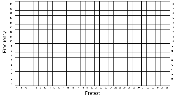
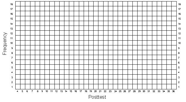
As before, you should graph the univariate distributions for the pretest and posttest in Figures 2-1 and 2-2. But here, unlike in the first exercise, the 50 people are randomly divided into two groups. It would be nice if you could distinguish the scores of these two groups in your graphs of the distributions. You should do this by using different colored pens or pencils and lines that slant in different directions for the program and comparison cases. For instance, let's say that the first four persons in Table 2-1 have the following pretest scores and group assignments:
| Person | Pretest X from Table 1-1 | Group Assignment Z |
|---|---|---|
| 1 | 12 | 1 |
| 2 | 12 | 0 |
| 3 | 10 | 0 |
| 4 | 12 | 1 |
In this case, the histogram for these four persons would look like
 .
.
Now plot the data for all 50 persons for both the pretest (Figure 2-1) and posttest (Figure 2-2) making sure to distinguish between the two randomly assigned groups both in color and in the angle of the mark you make. As in the first simulation, you should estimate the central tendency for both the pretest and posttest, but here you should do it separately for the program and comparison cases.
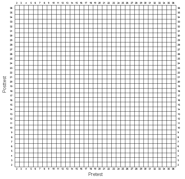
Now, plot the bivariate distribution in Figure 2-3. Again, you need to have a system for distinguishing between program and comparison cases when they fall in the same box. Use different colored pens or pencils for each. In addition, use different marks according to the following system:
First program case  ,
first comparison case
  ,
second program case
  ,
second comparison case
  .
So, if you have a pre-post pair that happens to have two program and two comparison cases,
the graph should look like
  .
.
Now, plot the lines on the bivariate plot that describe the pre/post relationship (as described in the first simulation exercise), doing a separate line for the program and comparison groups.
There are several things you should note. First, the pretest central values for the two groups should be similar (although they are not likely to be exactly the same). This is, of course, because the groups were randomly assigned. Second, the posttest central values should clearly differ. In fact, we expect that the difference between the average posttest values should be approximately the 7 units that you put in. In addition, the vertical difference between the relationship lines in the bivariate plot (Figure 2-3) should also be about 7 units.
At this point you should be convinced of the following:
- The design simulated here is a very simple single-factor randomized experiment. The single factor is represented by the 0,1 treatment variable that represents which group people are in. You could simulate more complex designs. For example, to simulate a randomized block design you would first rank all persons on the pretest. Then you could set the block size, for example at n = 2. Then, beginning with the lowest two pretest scorers, you would randomly assign one to the program group and the other to the comparison group. You could do this by rolling a die — if you get a 1, 2, or 3 the lowest scorer is a program participant; if you get a 4, 5, or 6 the higher scorer is. Continuing in this manner for all twenty-five pairs would result in a block design.
-
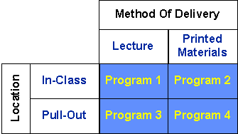
You could also simulate a 2×2 factorial design. Let's say that you wanted to
evaluate an educational program that was implemented in several different ways. You
decide to manipulate the manner in which you teach the material (Lecture versus Printed
Material) and where the program is given (In-class or Pull-out). Here you have two
factors — Delivery of Material and Location — and each factor has two
levels. We could summarize this design with a simple table that shows the
four different program variations you are evaluating:
Notice that we need a 2×2 table to summarize this study. Not surprisingly, we would call this a 2×2 factorial experimental design. If you were simulating this, you would actually have to randomly assign persons into one of the four groups. One advantage of this kind of design is that it allows you to examine how different program characteristics operate together (or "interact") to produce a program effect.
- You should recognize that the design simulated here can be considered a repeated measures experimental design because a pretest and posttest are used. You could simulate a posttest-only experimental design as well.
Randomized Experimental Design — Table 2-1
| Person | Pretest X from Table 1-1 | Group Assignment Z | Hypothetical Program Effect | Effect of Program (G) | Posttest Y from Table 1-1 | Posttest (Y) for Randomized Experimental Design |
|---|---|---|---|---|---|---|
| 1 | 7 | |||||
| 2 | 7 | |||||
| 3 | 7 | |||||
| 4 | 7 | |||||
| 5 | 7 | |||||
| 6 | 7 | |||||
| 7 | 7 | |||||
| 8 | 7 | |||||
| 9 | 7 | |||||
| 10 | 7 | |||||
| 11 | 7 | |||||
| 12 | 7 | |||||
| 13 | 7 | |||||
| 14 | 7 | |||||
| 15 | 7 | |||||
| 16 | 7 | |||||
| 17 | 7 | |||||
| 18 | 7 | |||||
| 19 | 7 | |||||
| 20 | 7 | |||||
| 21 | 7 | |||||
| 22 | 7 | |||||
| 23 | 7 | |||||
| 24 | 7 | |||||
| 25 | 7 | |||||
| 26 | 7 | |||||
| 27 | 7 | |||||
| 28 | 7 | |||||
| 29 | 7 | |||||
| 30 | 7 | |||||
| 31 | 7 | |||||
| 32 | 7 | |||||
| 33 | 7 | |||||
| 34 | 7 | |||||
| 35 | 7 | |||||
| 36 | 7 | |||||
| 37 | 7 | |||||
| 38 | 7 | |||||
| 39 | 7 | |||||
| 40 | 7 | |||||
| 41 | 7 | |||||
| 42 | 7 | |||||
| 43 | 7 | |||||
| 44 | 7 | |||||
| 45 | 7 | |||||
| 46 | 7 | |||||
| 47 | 7 | |||||
| 48 | 7 | |||||
| 49 | 7 | |||||
| 50 | 7 |
Randomized Experimental Design — Figure 2-1

Randomized Experimental Design — Figure 2-2

Randomized Experimental Design — Figure 2-3
