Regression Artifacts

In this exercise we are going to look at the phenomenon of regression artifacts or "regression to the mean." First, you will use the data from the original simulation and create nonequivalent groups just like you did in the Nonequivalent Group Design exercise. Then you will "match" persons from the program and comparison groups who have the same pretest scores, dropping out all persons for whom there is no match. You do this because you are concerned that the groups have different pretest averages, and you would like to obtain "equivalent" groups. Second, you are going to regraph the data for all 50 persons from the Generating Data (GD) exercise, to gain a deeper understanding of regression artifacts.

To begin, review what you did in the NEGD exercise. Starting with 50 pretest and posttest scores (each composed of a common true score and unique error components), you first made the groups nonequivalent on the pretest by adding 5 to each program person's pretest value. This initial difference was the same on the posttest, and so you added the same 5 points there. Finally, you included a program effect of 7 points, added to each program person's posttest score.

In this exercise, you will start with the data in the GD exercise, and will do the same thing you did in the NEGD exercise except that we will not add in a program effect. That is, in this simulation we assume that the program either was never given or did not work (i.e., the null case). The first thing you need to do is to copy the pretest scores from column 5 of Table 1-1 into column 2 of Table 5-1. Now, you have to divide the 50 participants into two nonequivalent groups. We can do this in several ways, but the simplest would be to consider the first 25 persons as being in the program group and the second 25 as being in the comparison group. The pretest and posttest scores of these 50 participants were formed from random rolls of pairs of dice. Be assured, that on average these two subgroups should have very similar pretest and posttest means. But in this exercise we want to assume that the two groups are nonequivalent and so we will have to make them nonequivalent. The easiest way to make the groups nonequivalent on the pretest is to add some constant value to all the pretest scores for persons in one of the groups. To see how you will do this, look at Table 5-1. You should have already copied the pretest scores (X) for each participant into column 2. Notice that column 3 of Table 5-1 has a number "5" in it for the first 25 participants and a "0" for the second set of 25 persons. These numbers describe the initial pretest differences between these groups (i.e., the groups are nonequivalent on the pretest). To create the pretest scores for this exercise, add the pretest scores from column 2 to the constant values in column 3 and place the results in column 4 of Table 5-1 under the heading "Pretest (X) for Regression Artifacts". Note that the choice of a difference of 5 points between the groups was arbitrary. Also note that in this simulation we have let the program group have the pretest advantage of 5 points.

Now you need to create posttest scores. You should copy the posttest scores from column 6 of Table 1-1 directly into column 5 of Table 5-1. In this simulation, we will assume that the program either has no effect or was never given, and so you will not add any points to the posttest score for the effect of the program. But we assume that the initial difference between the groups persists over time, and so you will add to the posttest the 5 points that describes the nonequivalence between groups. In Table 5-1, the initial group difference (i.e., 5 points difference) is listed again in column 6. Therefore, you get the final posttest score by adding the posttest score in column 5 and the group differences in column 6. The sum should be placed in column 7 of Table 5-1 labeled "Posttest Y for Regression Artifacts".

Now, just as you have done in previous exercises, plot the pretest and posttest frequency distributions in Figures 5-1 and 5-2, being sure to use different colors for the program (persons 1-25) and comparison (persons 26-50) groups. Also, estimate the central tendency for each group on both the pretest and posttest. You should notice that the average of the program groups is about 5 points higher than the average of the comparison group on both measures.

If you were conducting a nonequivalent group design quasi-experiment and obtained the pretest distribution in Figure 5-1, you would rightly be concerned that the two groups differ prior to getting the program. To remedy this, you might think it is a good idea to look for persons in both groups who have similar pretest scores, and use only these matched cases as the program and comparison groups. You might conclude that by only using persons "matched" on the pretest you can obtain "equivalent" groups.

You will match persons on their pretest scores, and put the matched cases in Table 5-2. To do this, first look at the pretest frequency distribution in Figure 5-1. Notice again that the comparison group tended to score lower. Beginning at the lowest pretest score and moving upwards, find the lowest pretest score at which there are both program and comparison persons. Most likely there will be more comparison persons than program ones at the first score that has both. For instance, let's imagine that the pretest score of 9 is the first score that has persons from both groups and that at this value there are two cases from the comparison group and one from the program group. Obviously you will only be able to find one matched pair--you will have to throw out the data from one of the comparison group person because there is only a single program group case available for matching. Since the dice used to generate the data yield random scores, you can simply take the first person in the comparison group (Table 5-1, persons 26-50) who scored a 9 on the pretest. Record that person's ID number in column 1 of Table 5-2, their pretest in column 2 and their posttest score in column 3. Next, find the program person (in Table 5-1, persons 1-25) who also scored a 9 on the pretest and enter that person's ID number in column 4 of Table 5-2, their pretest in column 5 and their posttest score in column 6. Then move to the next highest pretest score in Figure 5-1 for which there are persons from both groups. Again, find matched pairs, and enter them into Table 5-2. Continue doing this until you have obtained all possible matched pairs. Notice that you should never use the same person more than once in Table 5-2.

At this point, you have created two groups matched on the pretest. To do so, you had to eliminate persons from the original sample of 50 for whom no pretest matches were available. You may now be convinced that you have indeed created "equivalent" groups. To confirm this, you might calculate the pretest averages of the program and comparison groups. They should be identical.

Have you in fact, created "equivalent" groups? Have you removed the selection bias (of 5 points) by matching on the pretest? Remember that you have not added in a program effect in this exercise. If you successfully removed the selection difference on the pretest by matching, you should find no difference between the two groups on the posttest (because you only put in the selection difference between the two groups on the posttest). Calculate the posttest averages for the program and comparison groups in Table 5-2. What do you find?

Most of you will find that on the posttest the program group scored higher on average than the comparison group did. If you were conducting this study, you might conclude that although the matched groups start out with equal pretest averages, they differ on the posttest. In fact, you would be tempted to conclude that the program is successful because the program group scored higher than the comparison group on the posttest. But something is obviously wrong here--you never put in a program effect! Therefore, the posttest difference that you are finding must be wrong.

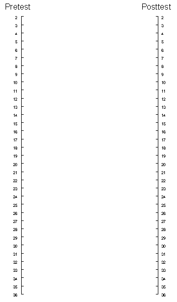
To discover what is wrong you will plot the data in Table 5-2 in a new way. Look at Figure 5-4 labeled "Pair-Link Diagram". Starting with only the comparison persons in Table 5-2, draw a straight line between the pretest and posttest scores of each person. Do the lines tend to go up, down, or stay the same from pretest to posttest? Next, using a different colored pen, draw the lines for the program group persons in Table 5-2. In which direction do these lines go? You should find that most of the program group lines go down while most of the comparison group lines go up from pretest to posttest. As a result of what you have seen, you should be convinced of the following:

• The average posttest difference between the program and comparison group is entirely due to regression artifacts that result from the matching procedure. Recall that because of the pretest difference of 5 points, which you put in, the entire program group had a higher pretest average than the entire comparison group. When you matched persons on the pretest, you were actually selecting the higher scoring comparison persons and the lower scoring program persons. Therefore, we expect the matched comparison group to regress down toward the entire group's mean and the matched program group to regress up toward the entire group's mean.
  
  
• In this simulation you made the program group higher on the pretest by adding 5 points. You should recognize that if the comparison group had been given this initial "advantage" the results of matching would have been reversed. In this case the matched comparison group would have had a higher posttest average than the matched program group. You would mistakenly conclude that the program was harmful--that is, even though the two matched groups start with equal pretest averages, the program group loses relative to the comparison group. Of course, any gain or loss is due to regression artifacts which result from a matching process that selects persons from the higher end of the distribution in one group and the lower end in the other.
  
  
• Matching should not be confused with blocking. If you had taken persons from two groups which differ on the pretest, matched them on pretest scores and then randomly assigned one of each pair to the program and comparison group, you would have equal numbers of advantaged and disadvantaged persons in each group. In this case, regression artifacts would cancel out and would not affect results.

Why do regression artifacts occur? We can get some idea by looking at a pair-link diagram for the entire set of 50 persons in the original Generating Data exercise. Draw the pair-links for each of the 50 persons of Table 1-1 on Figure 5-5. Recall that for this original set of data we had only one group (i.e., no program and comparison group), no selection biases and no program effects. You should be convinced of the following:

• Persons who score extremely high or extremely low on the pretest seldom do as extremely on the posttest. That is, there should be very few pair-link lines which go from a low pretest score to an equally low posttest score or which go from a high pretest score to an equally high posttest score.
  
  
• Recall that the pretest and posttest consists of two components, a true score which is the same on both tests and separate error scores for each. You should know that the regression artifact cannot be due to the true score. If you were to draw a pair-link diagram between the pretest and posttest true score, you would obtain nothing but horizontal lines (no regression) because it is the same for both tests. However, if you drew a pair-link diagram between the pretest error score and the posttest error score, you would see a clear regression effect. People with low pretest errors would tend to have higher posttest error scores and vice versa. This is because the pretest and posttest error scores were based on independent dice rolls, the two sets of error scores are random or uncorrelated. We can conclude that regression artifacts must be due to the error in measurement, not to the true scores.
  
  
• We can also view this in terms of correlations. First, assume that we have no measurement error-- persons always get the same score on the pretest and posttest. In this case, the pair-link diagram would only have horizontal lines, as stated above, and there would be no regression artifact. Furthermore, if people scored the exact same on both tests, there would be a perfect correlation between the two tests (i.e., r = 1). Next, assume that our pretest and posttest are terrible measures that only reflect error (i.e., they do not measure true ability, but do reflect random errors, at two points in time). Here, the two tests would be random or uncorrelated (i.e., r = 0). and we would expect maximum regression to the mean (i.e., no matter what subgroup you select on the pretest, the posttest average of that subgroup will always tend to equal the posttest average of the entire group). You should recognize that the more measurement error you have in the measures, the lower the correlation between the measures. Finally, you should also see that the lower the correlation between two measures the greater the regression artifact and, the higher the correlation the lower the regression.
  
  
• Finally, you should recognize that regression artifacts are purely a statistical phenomenon that results from a symmetric subgroup selection and imperfect correlation. This means that when we select a subgroup from the extreme of a distribution, we will find regression to the mean on any variable that is not perfectly correlated with the selection measure. This can lead the unwary analyst to some bizarre conclusions. For example, let us say you wanted to look at the effect of a special educational program that was given to all students in a school. Assume that you have pretest and posttest scores for everyone (but there is no control group). You would like to know whether subgroups in the school improved. First, you look at the students who scored low on the pretest. They appear to improve on the posttest (regression artifacts, of course). Next, you look at the students who scored high on the pretest. They appear to lose ground on the posttest. You might incorrectly conclude the education helps low scoring students but hurts high scoring students. Now let us say you decide to look at groups who differ on the posttest. The low posttest scorers did much better on the pretest. The high posttest scorers did much worse on the pretest. It almost appears as if students regress backwards in time. But by now you should recognize that this is simply a regression artifact that results from selection of groups on the extremes of the posttest and the imperfect correlation between the pretest and posttest.

Regression Artifacts Table 5-1

1	2	3	4	5	6	7
Person	Pretest X from Table 1-1	Pretest Group Difference	Pretest (X) for Regression Artifacts	Posttest Y from Table 1-1	Posttest Group Difference	Posttest (Y) for Regression Artifacts
1		5			5
2		5			5
3		5			5
4		5			5
5		5			5
6		5			5
7		5			5
8		5			5
9		5			5
10		5			5
11		5			5
12		5			5
13		5			5
14		5			5
15		5			5
16		5			5
17		5			5
18		5			5
19		5			5
20		5			5
21		5			5
22		5			5
23		5			5
24		5			5
25		5			5

Regression Artifacts Table 5-1
(cont.)

1	2	3	4	5	6	7
Person	Pretest X from Table 1-1	Pretest Group Difference	Pretest (X) for Regression Artifacts	Posttest Y from Table 1-1	Posttest Group Difference	Posttest (Y) for Regression Artifacts
26		0			0
27		0			0
28		0			0
29		0			0
30		0			0
31		0			0
32		0			0
33		0			0
34		0			0
35		0			0
36		0			0
37		0			0
38		0			0
39		0			0
40		0			0
41		0			0
42		0			0
43		0			0
44		0			0
45		0			0
46		0			0
47		0			0
48		0			0
49		0			0
50		0			0

Regression Artifacts Figure 5-1

Regression Artifacts Figure 5-2

Regression Artifacts Figure 5-3

Table 5-2
Matched Cases from Table 5-1

1	2	3	4	5	6
Comparison Group Person Number	Pretest X from Table 5-1	Posttest Y from Table 5-1	Program Group Person Number	Pretest X from Table 5-1	Posttest Y from Table 5-1
	Comparison Group Pretest Average=	Comparison Group Posttest Average=		Program Group Pretest Average=	Program Group Posttest Average=

Regression Artifacts Figure 5-4 Pair-Link Diagram

Regression Artifacts Figure 5-5 Pair-Link Diagram

Simulation Home Page